CS6670 : Project 1 - Daniel Lee (djl59)

CS 6670 Computer Vision

Project 1: Feature Detection and Matching

Questions to answer:

Describe your feature descriptor in enough detail that someone could implement

My custom descriptor is a fully implemented 5x5 pixels space assigned to each feature detected. Each pixel has a numerical value which is the magnitude of the second derivative of the image space. The magnitude is calculated as shown in (1)

(1)

(2)

The equation (2) is computed by convolving the image with a gradient kernel. However, since the feature detection is more robust for a smoothed image, it is preferred to have a smoothed image. However, since smoothing operation and derivation operation are both linear, they are associative. Therefore, in order to obtain the gradient of a smoothed image, it is valid to convolve the original image with a gradient of Gaussian kernel. Thus, is computed by convolving the original image with a derivative of a Gaussian kernel with respect to the x direction. The derivative of Gaussian is computed in MATLAB using gradient.m function, which outputs two gradient matrix in x and y direction. The numerical values are omitted here, but can be found in features.h file in the source code.

The second derivative of the image can be calculated by applying an additional gradient kernel. Simply, . However, since we already have the gradient of Gaussian, we can convolve with the gradient of the Gaussian twice, which will generate the second derivative of the twice smoothed original image (with Gaussian kernel).

My custom descriptor has similar initial steps as MOPS. It does use the orientation of the feature, and obtain the rotated region of interest. The acquisition of rotated image is done following these steps:

1. Using a rotation matrix, rotate a 100x100 pixels space around the feature. If this region is outside of the boundary, simply copy the value of the boundary. For example, if the 100x100 is outside of the top-right boundary, it will copy the intensity values from top and right boundary pixels.

2. The rotation will miss some pixels since pixel coordinates are in integer form. Therefore, fill in the missing pixels by taking the average of the surrounding 8 pixels.

3. Crop the middle 45x45 pixels.

Then, down-sample it to 5x5 pixel space by calculating (1). For example, in order to calculate the (0, 0) index of the descriptor, do the following:

1. Multiply the first 9x9 pixel space of the original image with magnitude square of 9x9 gradient of Gaussian both in x and y direction.

2. Add up all the numbers for x and y direction.

3. Compute (1), where is the summation you just calculated in the step above

Above steps are repeated for each 9x9 sub-regions of the 45x45 images (there are total 25 9x9 sub-regions in the 45x45 rotated image).

To conclude, my custom descriptor has a magnitude of the second derivative of the smoothed image using Gaussian kernel.

Explain why you made the major design choices that you did

A simple window descriptor is not robust to the rotation. MOPS descriptor does rotate the region of interest with an angle calculated from eigenvalue calculation, which represents the direction of the largest change. To make my descriptor somewhat robust to the rotation, the initial steps of rotating image was necessary. Then, the problem is how to represent the uniqueness of the feature. Simple 1-to-1 comparison of intensity value of the image is not robust to constant shifting or scaling. Also, the angle with respect to the plane is also difficult to solve without homography information. Once the region of interest is rotated to the same angle, the most efficient way of comparison would be the how intensity value changes within the region with respect to certain directions. Therefore, first or second derivative is selected to be evaluated. The first derivative gives somewhat reasonable information, but was not robust enough – it creates a large number of false positives. Then, second derivative was used to describe the feature. Second derivative is the derivative of the first derivative, and thus represents the uniqueness of the feature far better. And the actual performance was significantly better than the first derivative.

Report the performance

Here, ROC curves of feature comparison are presented. Two cases are studied: graf and Yosemite images. The graf images have translation AND rotation components, while Yosemite only has translation. ROC curve shows the performance of the feature matching. While the true homography information is given, it is possible to calculate the correct transformed pixel position from image 1 to 2. Using these correct values, ROC curve shows the evaluation result of the matching. A good feature matching algorithm should show a higher true positive rate with a small false positive rate. Along with the ROC curves, AUC values are presented for each descriptor and each comparison method. AUC means Area Under the Curve. 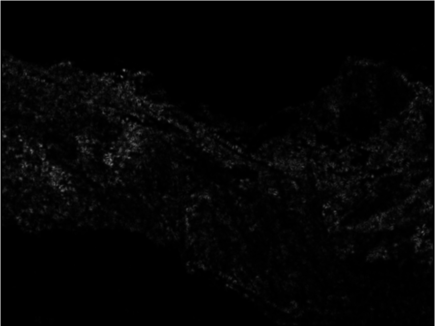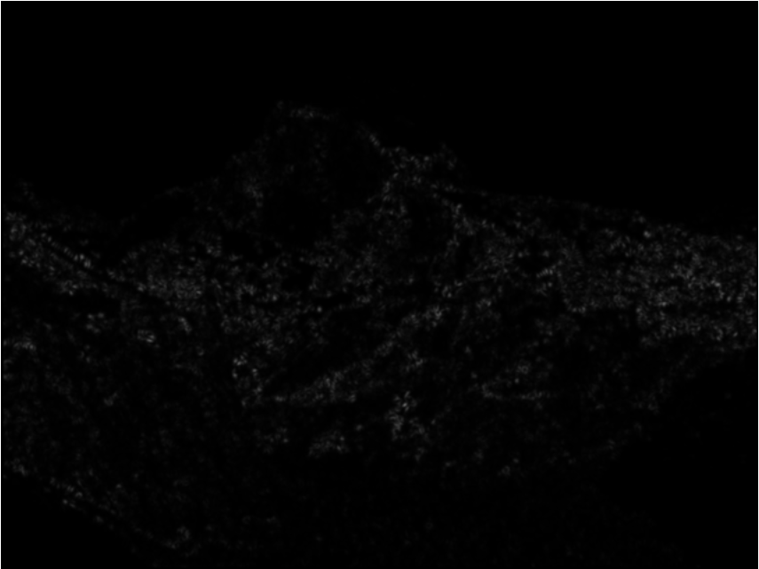Therefore, the higher AUC, the better performance feature matching did. Along with other plots, also two images for each graf and Yosemite image set, an image of Harris operator is presented. Please note that the actual Harris value was too small, so it needed to be up-scaled by the factor of 100. Yosemite graphics are rather large, but it is not resized for the originality of the picture.

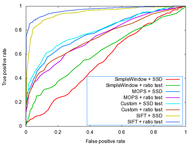
$Description: Description: E:\My Dropbox\School\Spring '11\CS6670\Project 1\Debug\pic\graf\results\plot.roc.png$

Figure 1 ROC curve of graf images with six different descriptors and 2 different methods used for feature matching

	SimpleWindow	MOPS	Custom
SSD Test	0.549302	0.783026	0.797184
Ratio Test	0.620259	0.740182	0.740142

Table 1 AUC results of feature matching with graf images

$Description: Description: E:\My Dropbox\School\Spring '11\CS6670\Project 1\Debug\harris.eps$

Figure 2 An Image of Harris operator for img1.ppm of graf pictures

$Description: Description: E:\My Dropbox\School\Spring '11\CS6670\Project 1\Debug\harris2.eps$

Figure 3 An Image of Harris operator for img2.ppm of graf pictures

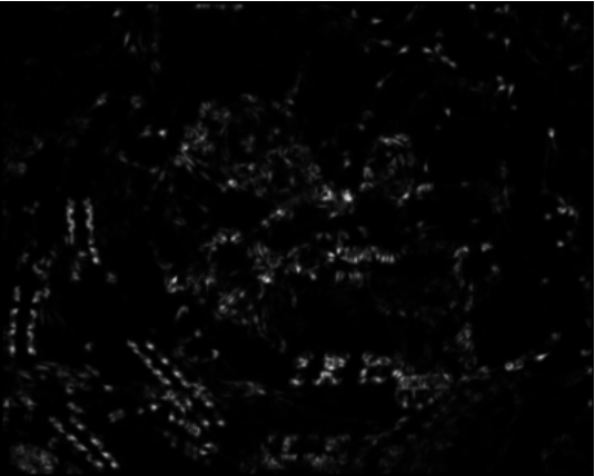
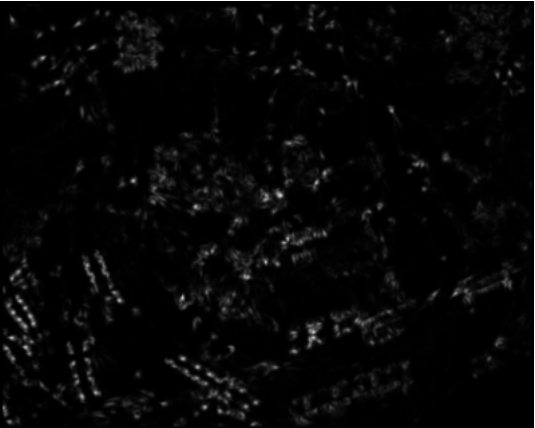
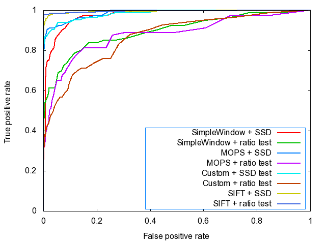
$Description: Description: E:\My Dropbox\School\Spring '11\CS6670\Project 1\Debug\pic\Yosemite\results\plot.roc.png$

Figure 4 ROC curve of Yosemite images with six different descriptors and 2 different methods used for feature matching

	SimpleWindow	MOPS	Custom
SSD Test	0.975227	0.986522	0.983423
Ratio Test	0.894571	0.878535	0.866802

Table 2 AUC results of feature matching with Yosemite images

$Description: Description: E:\My Dropbox\School\Spring '11\CS6670\Project 1\Debug\harris3.eps$

Figure 5 An Image of Harris operator for Yosemite1.jpg of Yosemite pictures

$Description: Description: E:\My Dropbox\School\Spring '11\CS6670\Project 1\Debug\harris4.eps$

Figure 6 An Image of Harris operator for Yosemite2.jpg of Yosemite pictures

Benchmark results are shown here for 4 different image sets: graf, bikes, wall, leuven

			graf	bikes	wall	leuven
Simple Window Descriptor	SSD Test	Average Error (pixel)	246.690682	377.465159	358.517751	387.398232
	SSD Test	AUC (-)	0.507024	0.391937	0.522764	0.376290
	Ratio Test	Average Error (pixel)	246.690682	377.465159	358.517751	387.398232
	Ratio Test	AUC (-)	0.542306	0.499773	0.559906	0.510037
Custom Descriptor	SSD Test	Average Error (pixel)	238.396335	261.378072	388.526983	340.994311
	SSD Test	AUC (-)	0.534563	0.662301	0.395809	0.315363
	Ratio Test	Average Error (pixel)	238.396335	261.378072	388.526983	340.994311
	Ratio Test	AUC (-)	0.539954	0.630166	0.546416	0.488659

Table 3 Benchmark results showing average error and AUC for four image sets. It was done on both simple and custom descriptor. The smaller values are better in average error, and larger is better in AUC comparison.

Each image sets have its own characteristics. graf has both translation and rotation in plane and in the view angle (like turning your head clockwise). wall images have little translation but vivid rotation in plane. bikes has almost no translation and rotation, but the images are blurred more and more. leuven images also have almost no translation and rotation, but the images are getting darker and darker. In graf, bikes, and leuven image sets, the custom descriptor showed improvement over the simple window descriptor. Especially in bikes and leuven, the custom descriptor shows much improvement. Therefore, the strength would be the robustness to the light condition / blurriness. The performance over the graf images is not significantly better and is worse over wall images. This means that the custom descriptor is not robust to the in plane rotation. Both graf and wall images have some in plane rotation and the performance is not good. Therefore, the weakness is the in plane rotation.

Custom Pictures Performance

Total 4 pictures are taken for performance test. All of them are from Memorial Hall in Willard Straight Hall in Cornell University. First two pictures have mostly about translation component. The second two pictures have in-plane rotation.

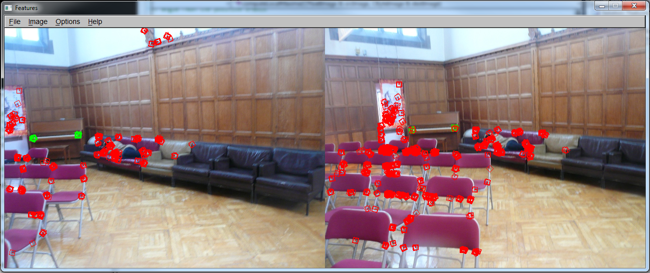
Two corners of the piano are selected. As shown in the right picture, it shows a good response for the matching. It successfully detected the piano corners on the right picture.

Some of the sofa corners and chair corners are selected. Also, one picture on the wall picture is selected too. On the right picture, it successfully found the wall picture, and some sofa corners. There are some false positives for the chair corners.

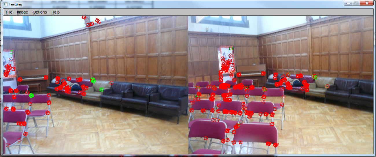
Obvious corners of these flags (which represent each college of Cornell) are selected. The performance is not great here.

Window corners and lamp corners are selected. It did find some of the features, but mostly failed. The middle white lamp’s features are not matched at all.

Above pictures show that the custom descriptor is not robust to the in-plane rotation. The first two pictures show some translation component, which it works well. However, in the bottom two pictures, which show in-plane rotation, the matching did not work out well.